What Quantization Really Does to LLM Accuracy

When you see a model name like “DeepSeek-V4-Flash-0731-UD-Q4_K_XL” or “Llama-3.3-70B-Instruct-Q4_K_M,” it reads like alphanumeric soup. Is a bigger number better? Is FP8 more efficient than Q4, or less? Either way, the label implies one setting, turned to one level, for the whole model.

That’s not what happens, and the gap between what the label says and what the model actually does is where most confusion about quantization lives.

This article closes that gap using two models as worked examples, chosen because they fail the same intuition in opposite directions.

DeepSeek-V4-Flash-0731 is the strange one. Its official checkpoint is already a deliberate FP4/FP8/BF16 mixture, because the model was trained to run at low precision rather than squeezed into it afterward. That single fact breaks most of the rules of thumb people carry around: its Q8 download is only 7 GB larger than its Q4, and converting it “back” to BF16 recovers nothing at all.

Llama 3.3 70B is the control. Conventionally trained in BF16, with 29 published quantization variants running from 141 GB down to 17 GB, it shows what a normal ladder looks like when you can see every rung laid out at once, and where even a normal ladder stops agreeing with its own labels.

By the end you should be able to answer:

why “FP8” or “four-bit” describes almost nothing on its own,
why quantization damage hides in conversation and surfaces in code,
why a four-bit model can outperform an eight-bit one,
why upcasting a low-precision checkpoint to BF16 recovers nothing,
and how to pick a rung on a download page for the work you actually do.

The short version, if you only want the rule: read the model’s configuration file (usually config.json), not just the filename. DeepSeek-V4-Flash-0731’s declares "expert_dtype": "fp4" for its experts, plus an FP8 quantization_config with "fmt": "e4m3" and 128×128 scaling blocks. That is the numeric layout the model actually runs in, and its filename mentions none of it. The rest of this explains why the filename can’t tell you.

What a model is, numerically

A trained language model is an enormous pile of numbers, hundreds of billions of them. Running it means multiplying and adding those numbers together, over and over, for every token it reads and every token it writes. (A token is a chunk of text, usually a word or a piece of one.)

Quantization is the decision about how precisely to write each of those numbers down.

Write them with fewer digits and the file shrinks, the memory bandwidth drops, and the math runs faster. Each number also becomes slightly wrong. The entire subject is about which errors you can afford.

The catch is that a model doesn’t have one pile of numbers. It has several kinds, they play different roles, and they don’t have to share a format:

Component	What it is	Common formats
Weights	What the model learned in training. Fixed once training ends.	BF16, FP8, FP4, INT8, INT4
Activations	The scratch work — values computed as your prompt flows through the layers.	BF16, FP16, FP8
Matrix-multiply inputs	The numbers actually handed to the GPU’s tensor cores.	BF16, FP8, FP4
Accumulators	The running totals inside a multiplication, before the answer comes out.	FP32, BF16
KV cache	A stored summary of every earlier token, so the model doesn’t recompute the past.	BF16, FP8, INT8, INT4

There’s a shorthand for the two that get discussed most. W is weights, A is activations, and the number after each is its bit width. W8A16 means eight-bit weights with sixteen-bit activations. W4A4 means both dropped to four.

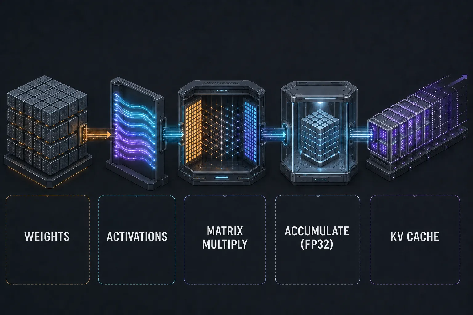
Five connected pipeline modules — weights, activations, matrix multiply, accumulation, KV cache — each drawn with a different grid density to signal a different numerical precision.

So “FP8” alone leaves most of the question open. FP8 weights with BF16 activations is W8A16. Both in FP8 is W8A8. Maybe the weights stayed BF16 and only the KV cache went to FP8. Maybe the hardware multiplies FP8 inputs but keeps the running totals in FP32. Maybe most layers are FP8 and a handful of delicate ones stayed BF16.

People call all of those “FP8 inference.” They do not behave the same.

So look past the bit count and ask:

Which values are being compressed, how are they being compressed, and was the model trained to operate that way?

That last question turns out to matter enormously, and it’s why DeepSeek-V4-Flash-0731 makes such a useful case study. Its official checkpoint is already a deliberate mix of FP4, FP8, and BF16. The compression isn’t something a third party did to it afterward; it’s how the model was built.

What quantization actually changes

Say one of a model’s weights is:

w = 0.183742

A low-precision format has a fixed menu of numbers it can represent, a grid of allowed values with gaps in between. If 0.183742 doesn’t land on that grid, the format stores the closest value it has:

\hat{w} = 0.1875

The gap between what you wanted and what got stored is the quantization error:

\epsilon = \hat{w} - w

A precise value on a continuous ruler snapping to the nearest step of a coarse grid, with a small glowing gap marking the quantization error, expanding into a field of billions of tiny grid points.

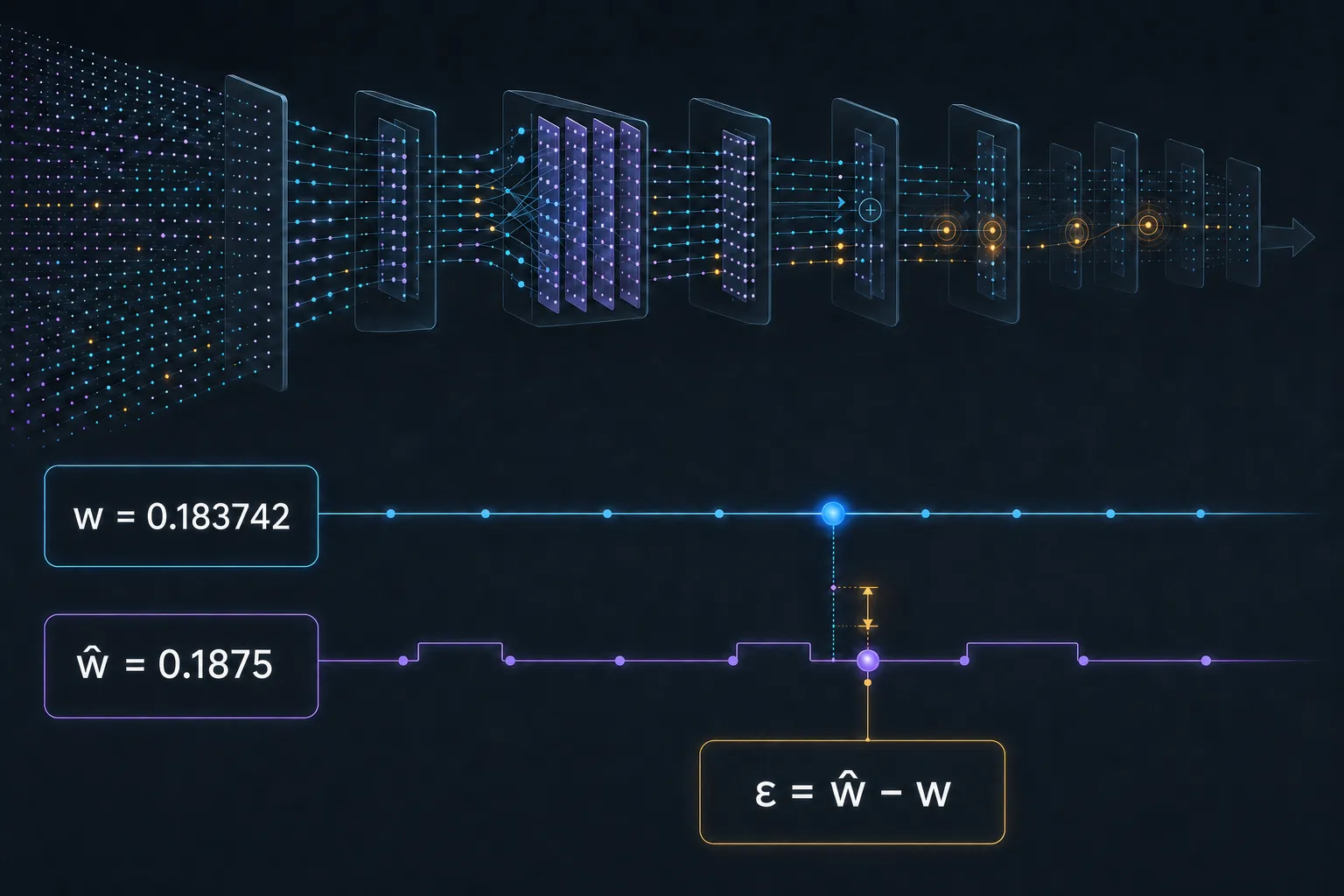
For a single weight, that error is trivial. Nothing depends on the fifth decimal place of one number out of 300 billion.

But a transformer performs billions or trillions of multiply-add operations per token, and errors that small do several different things across a network that size:

Many cancel each other out, since the errors point in random directions.
Many stay too small to change anything downstream.
Some accumulate along a path, growing rather than canceling.
Some reorder attention scores, changing what the model looks at.
Some flip which expert a routed model sends the token to (more on that below).
Some reorder two nearly tied candidates for the next token.

That last one deserves a closer look, because it’s the reason quantized models are so easy to misjudge.

Why two completions can differ without either being worse

At the end of every step, the model produces a raw score for every token in its vocabulary. Those scores are called logits, and the highest one (or a sample weighted by them) becomes the next token.

Suppose a forward pass ends like this:

"therefore" logit: 12.482
"however"   logit: 12.479

Three thousandths apart. A rounding error anywhere upstream can flip that order.

So the quantized model writes “however,” whereas the original model writes “therefore.” Every token after that is generated from a different prefix, and the two answers can diverge into completely different paragraphs, all from a numerical difference far too small to call a defect.

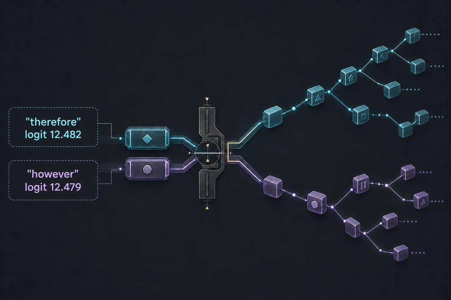
Two nearly tied token candidates passing a selection gate; a tiny nudge puts one ahead, and the generation path splits into two increasingly different but equally coherent branches.

Both phrasings can be equally correct and equally well reasoned. Text generation is chaotic in the mathematical sense: tiny early differences produce large late ones, and that says nothing by itself about quality.

Which means you cannot evaluate a quantization by putting two completions side by side and reading for differences. You will always find differences. Almost everyone’s first instinct is that side-by-side, and it answers nothing; you have to measure outcomes across a meaningful set of tasks instead.

The precision ladder is not a quality ladder

It’s tempting to line the formats up as a simple ranking:

FP32 is best, BF16 is a bit worse, FP8 worse again, and four-bit formats are much worse.

That model is too simple, and to see why, you need to know what those bits are actually doing.

How a floating-point number is built

Floating point is scientific notation in binary. When you write 3,500 as 3.5 × 10³, you’ve split the number into digits (3.5) and magnitude (10³). Floating-point formats do the same thing with three fields:

the sign bit — positive or negative,
the exponent bits — how large or small the number is, which sets the range,
the fraction bits (also called mantissa or significand) — the actual digits, which set the precision.

That split is the key to the whole subject. Exponent bits buy range, meaning how far the format reaches from the tiniest values to the largest. Fraction bits buy resolution, meaning how finely it distinguishes numbers sitting close together.

A format with too little range overflows to infinity or collapses to zero. A format with too little resolution smears nearby values into the same number. Those are different failures, and formats of the same total size can trade between them very differently.

FP32: the numerical reference

FP32 spends its 32 bits on:

1 sign bit
8 exponent bits
23 fraction bits

Broad range, high resolution inside that range. It’s what “just use full precision” usually means.

It’s also brutally expensive at scale. A 304-billion-parameter model stored entirely in FP32 needs roughly:

304\text{B} \times 4\text{ bytes} = 1.216\text{ TB}

That’s weights alone, before the KV cache, activations, and runtime buffers.

FP32 still earns its place for keeping master weights during training, for accumulating sensitive operations, and for producing reference results to check other formats against. For ordinary inference, storing every weight in it buys almost nothing.

BF16: the practical reference

BF16 spends its 16 bits on:

1 sign bit
8 exponent bits
7 fraction bits

Look at the exponent field: 8 bits, the same as FP32. BF16 was designed by taking FP32 and throwing away fraction bits while keeping the full range. It reaches just as high and just as low as FP32 does; it simply can’t split hairs as finely between neighboring values.

That’s the right trade for neural networks, where activations occasionally spike to extreme magnitudes and the cost of overflow is catastrophic while the cost of a slightly blurry value is negligible.

A BF16 copy of that same 304-billion-parameter model needs about 608 GB of weights. When kernels and accumulators are implemented properly, BF16 inference is close enough to FP32 that the difference is usually unmeasurable, which is why BF16, rather than FP32, is the practical baseline everything else gets compared against.

FP16 trades the opposite way

FP16 splits its 16 bits differently:

1 sign bit
5 exponent bits
10 fraction bits

Three fewer exponent bits, three more fraction bits. Same total size, opposite priorities: FP16 resolves nearby values more finely than BF16, and runs out of range far sooner.

Those three exponent bits matter more than they look. Each one roughly squares the reachable magnitude, so FP16 tops out around 65,504 while BF16 reaches into the 10³⁸ range. Train a large model in FP16 without loss scaling and gradients underflow to zero or activations overflow to infinity; that fragility is exactly what BF16 was invented to remove.

For inference the two usually produce comparable quality, and BF16 is simply harder to blow up.

FP8 lives or dies by scaling

Two FP8 layouts are in common use:

E4M3 — 4 exponent bits, 3 fraction bits. Favors precision.
E5M2 — 5 exponent bits, 2 fraction bits. Favors range.

With eight bits total, neither has much of either. E4M3 reaches about ±448 at the top, which sounds workable until you remember it has to cover the very small values in the same tensor too. Round a real tensor straight into FP8 and much of it piles into the same few buckets or falls off the ends of the range.

The fix is scaling, and it’s the same idea as picking sensible units. Describing a coin in kilometers wastes every digit you have. Switch to millimeters and the same digits suddenly carry real information.

A scale factor does that numerically. Instead of storing 0.0012, 0.0034, and 0.0021 in a format that barely reaches down there, store one shared multiplier (say 0.001) and then keep 1.2, 3.4, and 2.1 in the middle of the format’s comfortable range. Multiply back at compute time.

The finer the granularity of those scales, the better each group fits. Scales can be assigned:

per tensor — one multiplier for the whole thing, crude,
per channel — one per row or column,
per token — one per position in the sequence,
or per block — one for each small tile of values.

Do this well, and FP8 inference tracks BF16 remarkably closely. A large study of Llama 3.1 models found FP8 W8A8 effectively lossless across the scales it evaluated, while well-tuned INT8 W8A8 showed roughly 1–3% degradation.

That isn’t a promise that FP8 is always free. It’s evidence for something more useful:

How you quantize can matter as much as how many bits you use.

Four-bit formats need every trick at once

Four bits give you 16 possible values, and that’s the entire menu before scaling enters the picture. A tensor of weights spanning several orders of magnitude has to be squeezed onto it.

At that point, block scaling becomes mandatory rather than helpful. Formats like MXFP4 pair a tiny element format (commonly E2M1: one sign bit, two exponent bits, one fraction bit) with a scale factor shared across a small block of values, typically 32 of them. Each block gets to sit in its own numerical neighborhood.

Even with that, converting every tensor to four bits usually wrecks the model. Four-bit inference works when several techniques cooperate:

small quantization groups, so each scale covers a narrow range,
carefully chosen scales rather than naïve min/max,
explicit handling of outlier values,
keeping the most sensitive tensors at higher precision,
quantization-aware training,
or post-training algorithms such as AWQ and GPTQ that use calibration data to pick better roundings.

There’s a reliable pattern in which four-bit setups survive. A weight-only INT4 model often stays impressively capable, because the weights are the only thing compressed. Activations stay BF16, accumulators stay FP32, and every multiplication still has one high-precision operand. A naïvely converted W4A4 model tends to collapse, because both sides of every multiplication have been gutted and the errors compound instead of canceling.

Where quality actually starts to fall

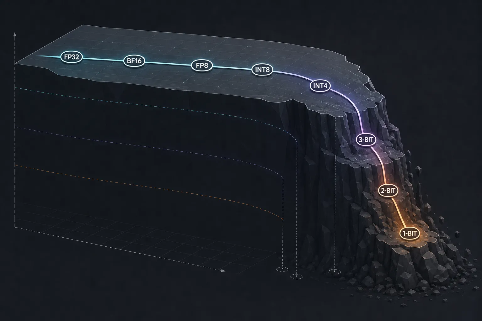
A terrain shaped like a performance curve: a broad flat plateau across high and medium precision, then a sharply nonlinear cliff as precision drops toward one bit.

For a conventional dense transformer trained in BF16, of which Llama 3.3 70B is our reference case, this is a reasonable starting expectation:

Inference configuration	Expected quality relative to BF16	Main qualification
FP32	Essentially identical	Much greater memory use
BF16	Reference quality	Common deployment baseline
FP16	Usually essentially identical	Narrower numerical range
FP8 W8A8	Often near-reference	Requires good scaling and kernels
INT8 W8A8	Usually a small measurable loss	Sensitive to activation outliers
INT8 or FP8 W8A16	Often extremely close	Less acceleration than W8A8
INT4 W4A16	Often usable to very good	Strongly dependent on model and task
FP4 W4A8 or W4A16	Can be very good when trained for it	Risky as a naïve conversion
W4A4	Significantly more fragile	Reasoning and exact output suffer
3-bit	Noticeably task-dependent	Coding and long context often degrade first
2-bit	Frequently substantial degradation	Style may survive after reasoning weakens
1–1.5-bit	Experimental or architecture-specific	Not a safe generic conversion

Read down that table, and you’ll notice the damage doesn’t arrive gradually. Sixteen bits to eight often costs nothing measurable. Four bits to three can fall off a cliff. Bartowski’s notes on the Llama ladder track the same shape from the practitioner’s side: everything down to Q4_K_M carries a “recommended,” Q3_K_M is bluntly labeled “low quality,” and the bottom rungs come with warnings.

The reason is that quantization doesn’t degrade a network the way turning down a volume knob does. Each layer learns to distinguish between values, and as long as the format can still represent those distinctions, the layer keeps working essentially as trained. The moment the grid gets too coarse to separate the values the layer needs to separate, that layer stops doing its job, and everything downstream inherits the failure.

So there’s a plateau, then a threshold, then a fast decline. The exact position of the threshold depends on the model, the layer, and the task, which is why nobody can hand you a universal bit count that’s “safe.”

Why architecture changes the answer

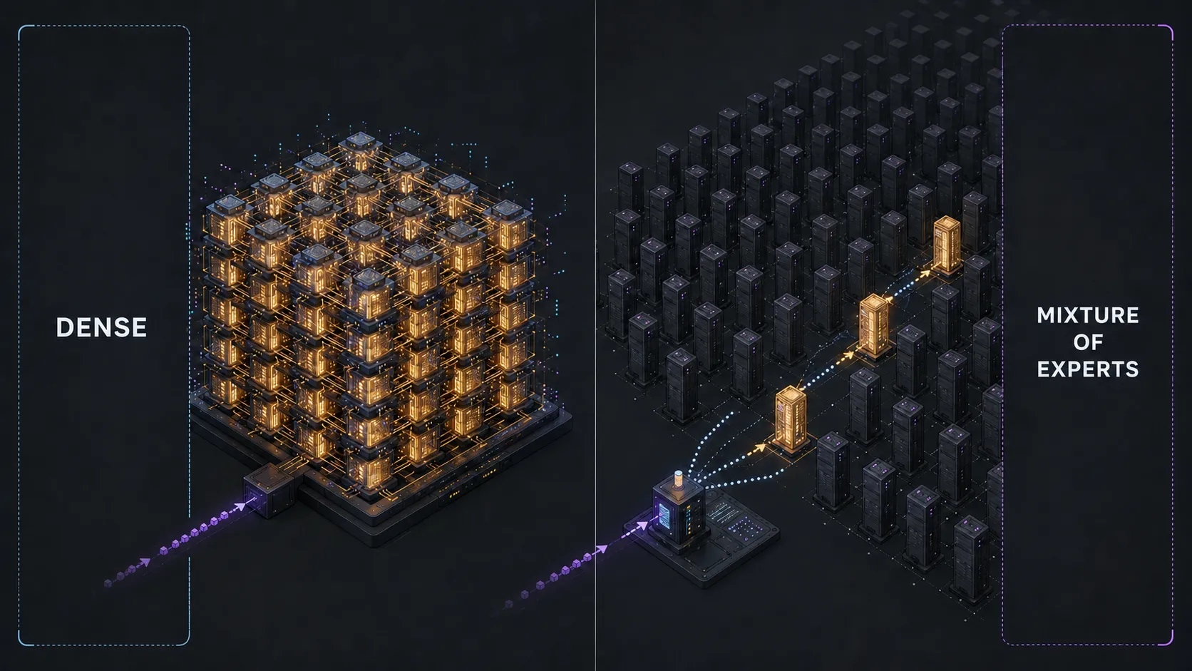
Split view: a dense transformer as a grid where every chamber lights up for every token, beside a mixture-of-experts city where only a few of hundreds of towers light along one token's path, directed by a small routing tower.

A quantization scheme that suits one model family can be a poor fit for another, and the biggest divide is between dense models and mixture-of-experts models.

Dense transformers spread the error everywhere

In a dense transformer, essentially every weight participates in computing every token. There’s no idle capacity. Quantization noise therefore spreads evenly through the entire network, and no single component carries disproportionate risk.

That evenness is why weight-only INT4 works as well as it does here. The weights are four-bit, but the rest of the path stays precise:

activations remain BF16 or FP16,
accumulators remain BF16 or FP32,
each small group of weights carries its own scale,
and outlier channels can be handled separately.

Dense Llama, Qwen, Gemma, and Mistral variants all tend to behave this way.

Mixture-of-experts models create a different opportunity

A mixture-of-experts (MoE) model splits its bulk into hundreds of separate weight blocks called experts, plus a small component called the router that picks a handful of them for each token. The rest sit idle for that token and still take up memory.

It’s tempting to call the experts specialists, but that oversells what’s going on. Nobody assigned them topics. The division of labor emerged during training, and for the most part nobody can say what any individual expert handles.

The result is a lopsided distribution: the expert matrices hold the overwhelming majority of the parameters, only a few run per token, and the routers, attention layers, and shared components are comparatively tiny.

This makes the experts the obvious compression target. A designer can push that enormous expert population down to four bits while keeping the small, sensitive machinery at higher precision: routers, attention layers, normalization parameters, embeddings, output layers, and selected activations.

The router needs special care, though, and the reason generalizes well beyond MoE.

Quantize an expert’s weights, and that expert’s output shifts slightly. Quantize the router and the token can be sent to a different expert entirely: a separate subnetwork with its own learned behavior, doing something else with the input. Since nobody labeled what these experts do, there’s no reason to expect the substitute to be a near-equivalent.

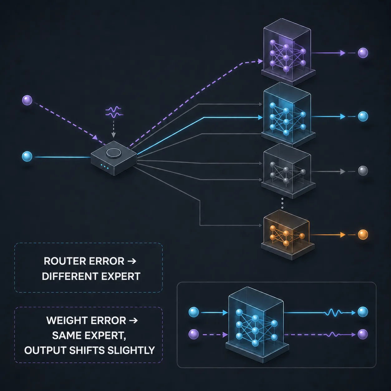
A token at a routing junction: one tiny perturbation switches it onto an entirely different expert track, contrasted with a small perturbation that only slightly changes output inside the chosen expert.

The first is an error in a value; the second is an error in a decision. Errors in decisions don’t average out, they branch. Any component whose output selects a path rather than contributing a number carries this same amplified risk.

Reasoning and code expose errors that conversation hides

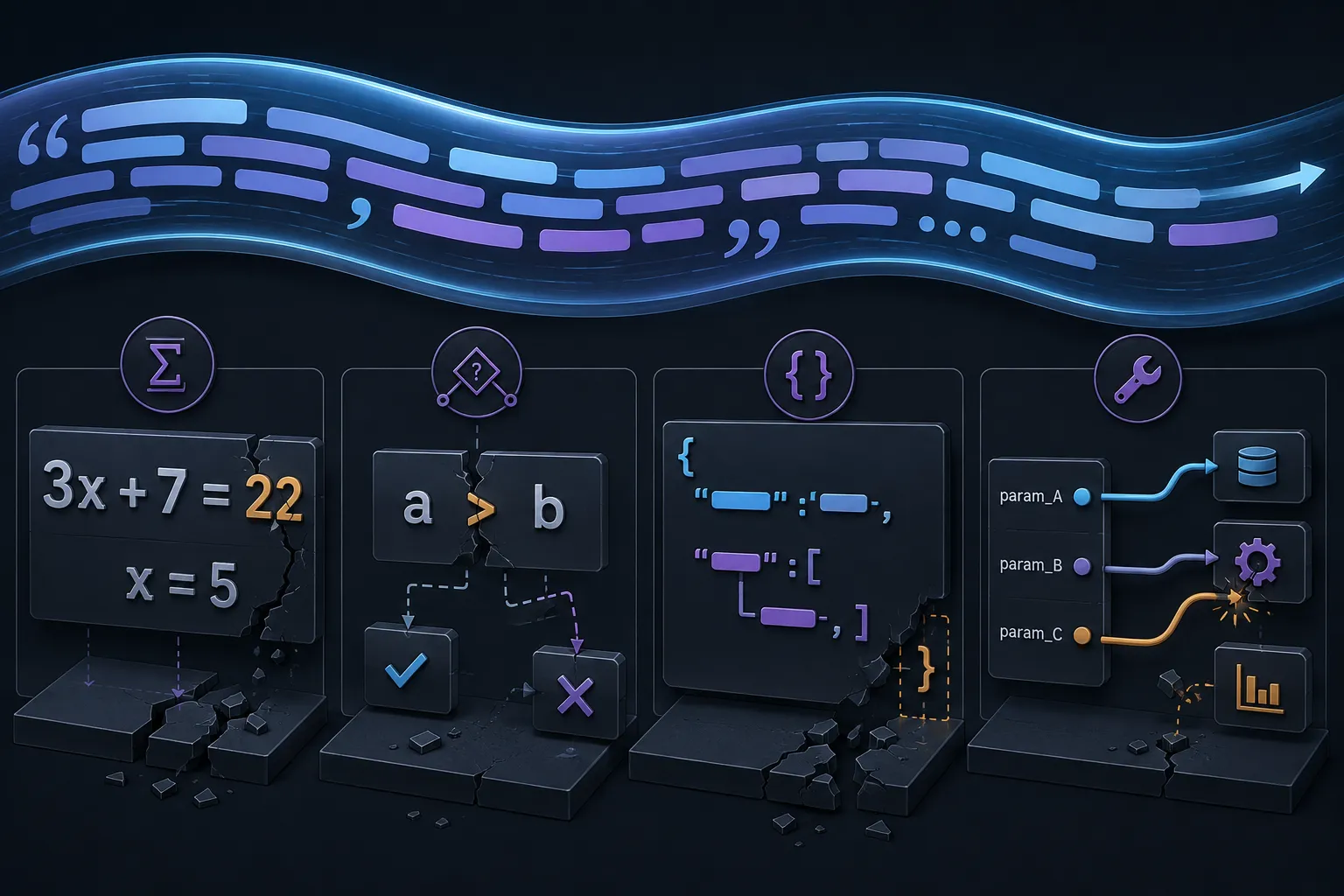
$A polished stream of prose flows smoothly across the top while beneath it exact structures fracture — a wrong digit, a reversed comparison, a missing brace, a misdirected tool parameter.$

Chat benchmarks flatter heavily quantized models, and understanding why is what keeps you from being fooled by your own testing.

Natural language is enormously redundant. Swap an adjective, reorder a clause, shift the tone a little, and the response still means what it meant. There are many acceptable ways to say the same thing, so small perturbations land on other acceptable outputs.

Exact work has no such cushion. A small numerical change can flip one digit in a calculation, reverse a comparison operator, rename a variable, drop a closing brace, misfill a tool parameter, or break one intermediate step of a proof. There’s one right answer and the perturbation moved you off it. Worse, in a chain of reasoning, every later step inherits the error and builds confidently on top of it.

Research on aggressive W4A4 and KV4 quantization finds that failures cluster around low-entropy tokens, the ones where the model was nearly certain, like digits and operators. That’s a striking result, and it makes sense on reflection: those are exactly the positions where a specific token is required and no paraphrase will do.

The practical consequence is that a quantized model can keep sounding articulate and confident long after it stopped being reliable at anything exact. Fluency is the last capability to degrade, so fluency is the worst possible thing to measure.

Long context makes KV-cache precision its own problem

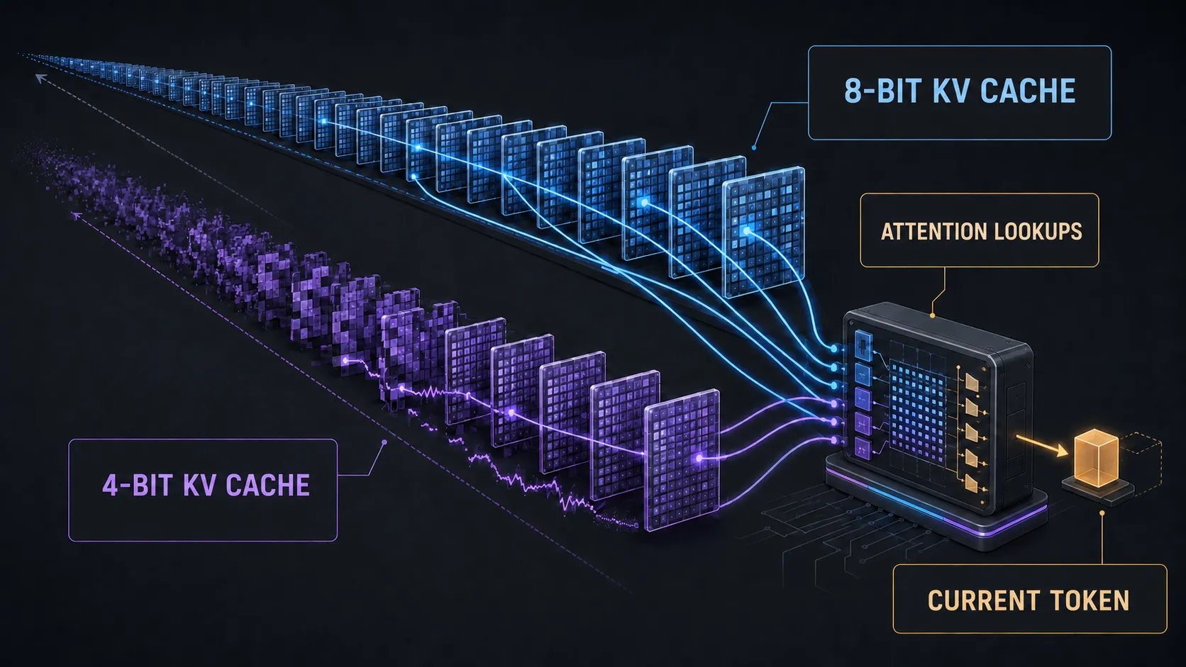
A model consulting a long archive of memory tiles that grow coarser with distance, shown as two parallel paths: a relatively safe eight-bit cache and a more fragile four-bit cache.

Weight precision gets the attention, but it isn’t the only place quality leaks out.

As the model reads, it computes a key and a value for every token and stores them, so it never has to recompute the past. That store is the KV cache, and every new token consults it all through attention. In long contexts, it grows large enough to dominate memory, making it an obvious target for compression.

The complication is that the KV cache is read constantly. A weight error gets applied once per layer; a KV-cache error gets re-read by every subsequent token, for as long as the conversation lasts.

Eight-bit KV caches are usually fairly safe, and four-bit is a gamble. One broad, long-context study found an average degradation of around 0.8% at eight bits, while some four-bit configurations lost as much as 59% on particular long-context tasks.

Results varied widely across models, tasks, and languages, but the lesson holds: “four-bit model” isn’t a precise enough description to predict behavior. Four-bit weights with a BF16 cache is a different machine from four-bit weights with a four-bit cache.

Why DeepSeek-V4-Flash-0731 is a different kind of case

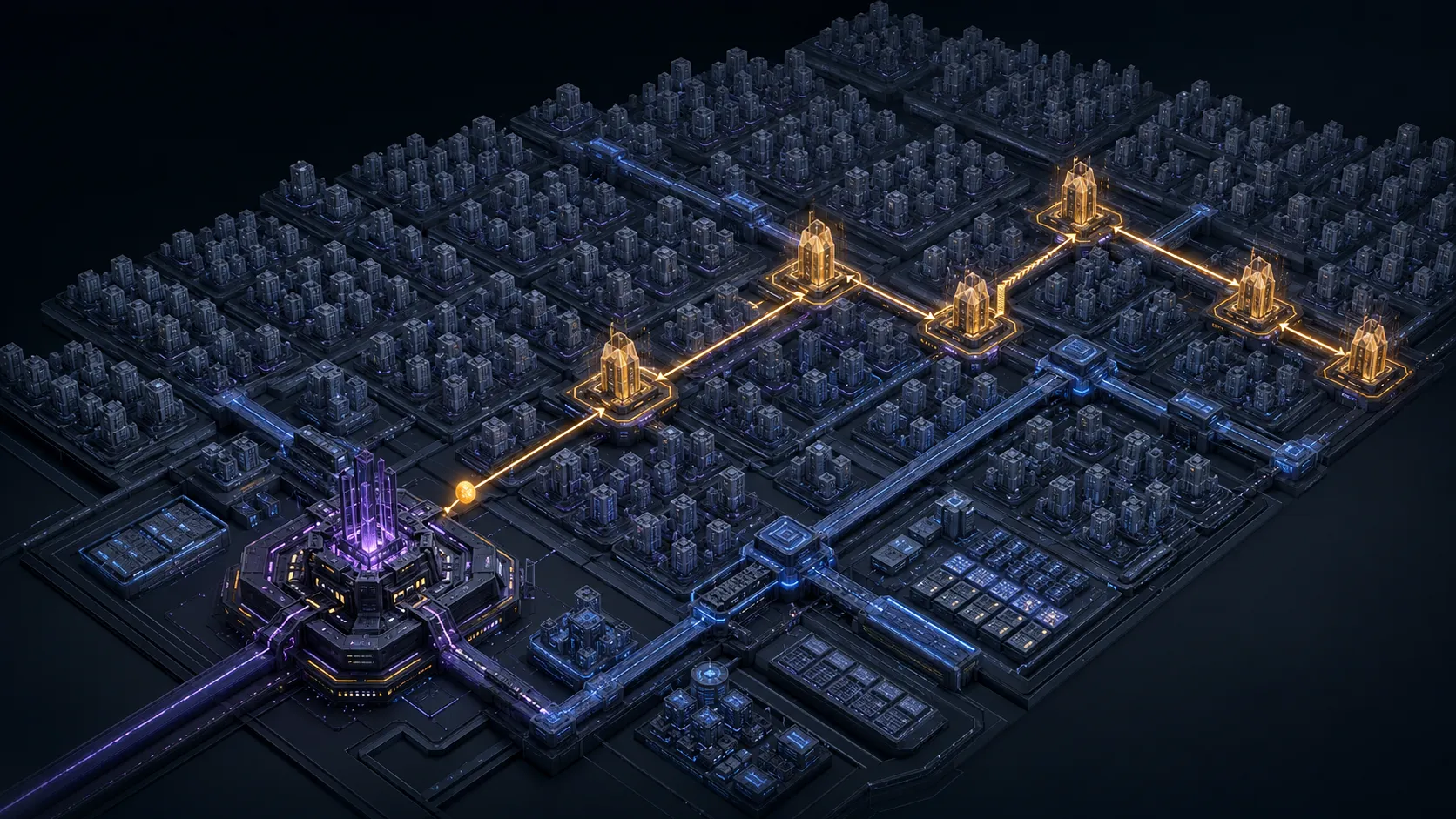
A mixture-of-experts model as a computational city: vast four-bit expert districts, eight-bit shared infrastructure, a few dense high-precision control centers, and one token's route lit through just six towers.

Everything so far assumed the normal situation: a model trained at high precision, then compressed afterward by someone else. DeepSeek-V4-Flash-0731 inverts that assumption, and the consequences run through every format decision below.

The official DeepSeek-V4-Flash-0731 checkpoint is already the low-precision reference model.

There is no BF16 original sitting behind it that a third party squashed. The released configuration declares a mixed-precision design on purpose:

FP4 routed-expert weights,
a broader FP8 quantization scheme,
FP8 E4M3 values,
dynamic activation quantization,
128×128 weight-scaling blocks,
BF16 as the general PyTorch dtype,
256 routed experts,
and 6 experts selected per token.

DeepSeek describes the V4 architecture as roughly 284 billion parameters with about 13 billion active per token and a one-million-token context window. The Hugging Face repository reports roughly 304 billion parameters for the 0731 release; the gap from the paper’s 284 billion appears to be the attached speculative-decoding components. The whole repository occupies about 167 GB.

Set that 167 GB against what uniform storage of 304 billion parameters would cost:

Format	Raw weight size
FP32	1,216 GB
BF16 or FP16	608 GB
FP8 or INT8	304 GB
FP4 or INT4	152 GB

At 167 GB, the checkpoint averages roughly 4.4 bits per parameter, before metadata and layout overhead. It lands just above the FP4 row, which tells you the composition immediately: the routed experts hold the overwhelming majority of the parameters and already sit at four bits, with the small remainder kept higher.

Nobody compressed this model to get there. It was built at 4.4 bits.

How can a model use FP4 without collapsing?

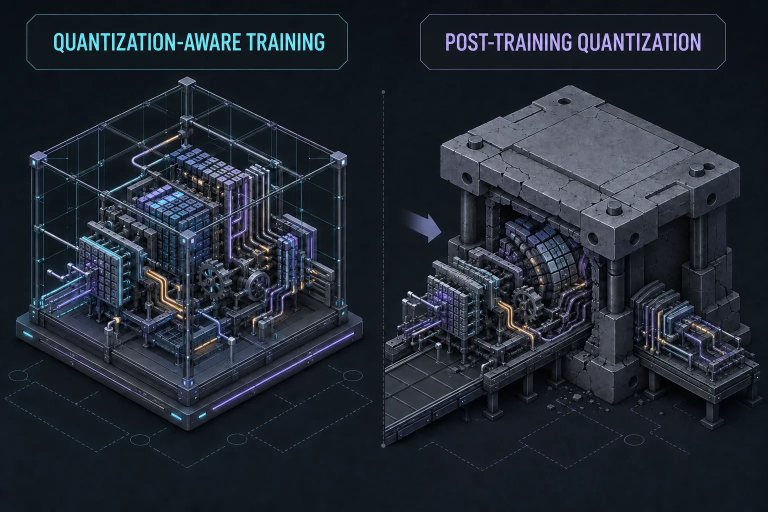
Side by side: a machine trained inside a restrictive low-precision framework emerges elegant and functional, while a finished high-precision machine forced through a compression mold afterward shows distortion.

Everything above said that naïve four-bit conversion wrecks models. So how does DeepSeek ship four-bit experts and stay competitive?

The answer is quantization-aware training (QAT), and the distinction between it and ordinary post-training quantization is the single most important idea in this article.

Post-training quantization builds the machine at full precision, then squeezes it into a smaller box afterward. The rounding happens once, at the end, and the model has no say in it. Whatever the weights happened to be, that’s what gets rounded, and whatever error results is the error you live with.

Quantization-aware training builds the machine inside the smaller box from the beginning. During training, the forward pass rounds the weights to the target format, so the model genuinely experiences being four-bit while it learns, while the optimizer keeps updating a higher-precision master copy behind the scenes.

That arrangement sounds contradictory, and resolving it is the clever part. Training works by computing, for every weight, a signal that says which direction to nudge it and how hard. Rounding destroys that signal: nudge a weight a little and it usually rounds to the same four-bit value, so the measured effect of the nudge is exactly zero and learning stalls immediately.

The standard trick is to compute that signal as though no rounding happened, then apply it to the high-precision master copy. The model gets judged on its rounded behavior but learns in smooth steps.

The payoff is that training can actively compensate. Weights drift toward values the four-bit grid represents well. Layers learn to tolerate the error their neighbors introduce. Errors get arranged so they cancel rather than compound. None of that is available to a converter running once on a finished model.

For DeepSeek V4 specifically:

MoE expert weights use MXFP4.
The sparse-attention indexer’s query/key path also runs at low precision.
Higher-precision master weights were quantized during training, not after.
The deployed checkpoint contains native FP4 expert weights.
Sensitive scores and operations stay at BF16 or above.

DeepSeek reports that the indexer’s reduced-precision scoring path kept roughly 99.7% recall on the KV entries it selects, while making the selector faster.

Whether every one of those choices holds up on every future workload is a fair question, and nobody has answered it comprehensively. But architecturally this is a different thing from downloading a BF16 model, running a generic four-bit converter, and hoping. DeepSeek V4 was trained around the representation it ships in. The quantization is part of the design, not a packaging step applied at the end.

Why converting it back to BF16 cannot recover accuracy

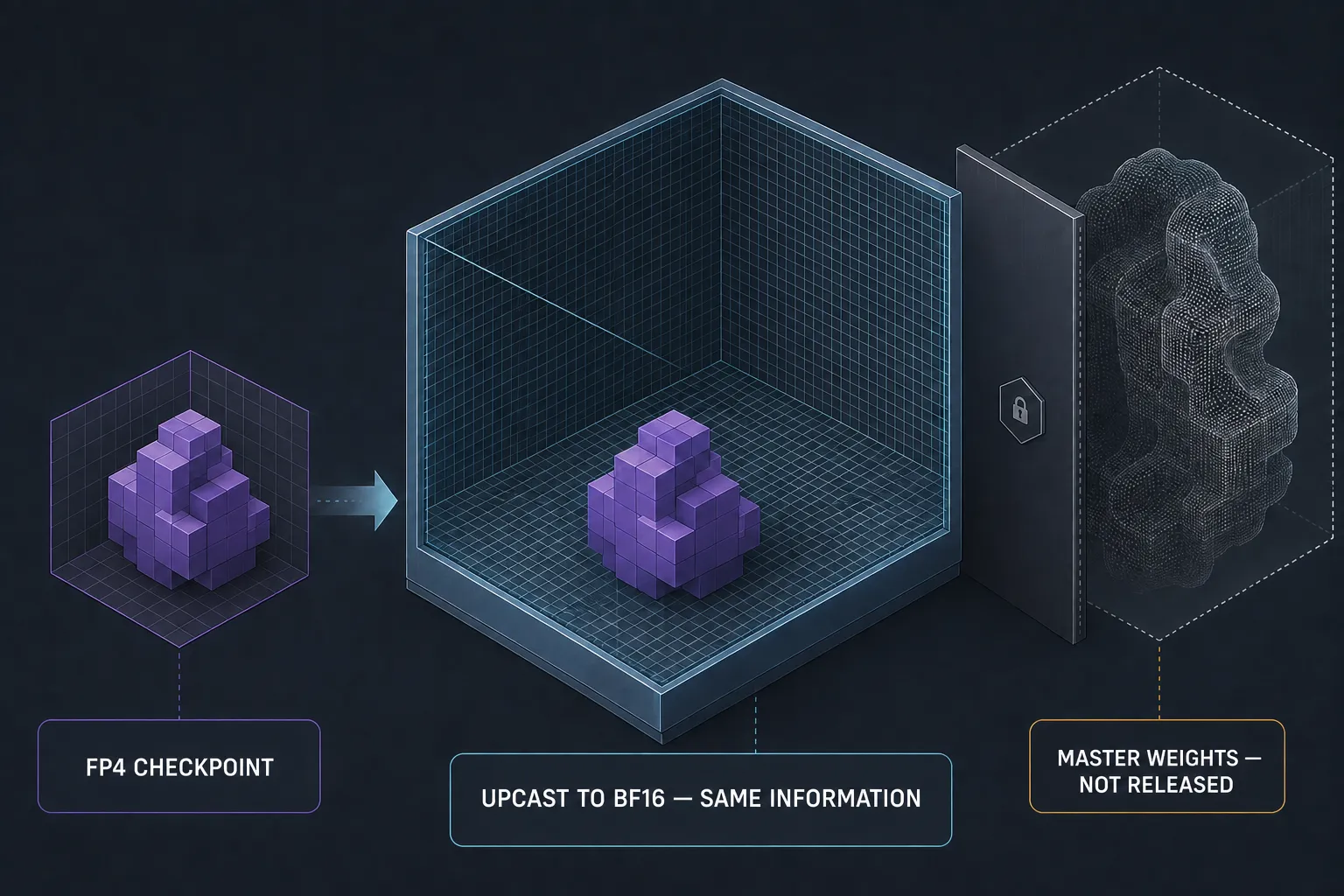
An object built from coarse four-bit blocks placed into a much finer high-precision container — the container can hold exquisite detail, but the object stays coarse; the detailed original fades behind an inaccessible barrier.

A natural thought: if four bits is lossy, convert the checkpoint up to BF16 and get the quality back.

It doesn’t work, and being precise about why explains a lot about what a checkpoint actually contains.

Suppose an FP4 expert weight in the official checkpoint holds:

1.5

A runtime can load that into BF16 and represent 1.5 beautifully. What it cannot do is recover what the high-precision master weight was during training. Was it 1.47? 1.51? 1.56? All of them round to the same stored value, and the checkpoint keeps no record of which one it was.

Converting a low-precision value into a larger type stores the same value more spaciously. It does not reconstruct information that was never in the file.

The distinction is between capacity and information. BF16 has more capacity, but you can’t fill it with anything you don’t have. Photographing a blurry photo at higher resolution gives you a bigger file of the same blur.

Upcasting the FP4 tensors to BF16 is still useful for one thing: running on hardware without native FP4 support. What it buys you is compatibility. What it costs is:

much higher memory consumption,
much higher bandwidth demand,
and essentially unchanged output quality.

So treat the official FP4/FP8/BF16 mixture as the model’s reference-quality form. Readers often assume a better BF16 edition exists somewhere behind it, waiting to be restored; for this model, none was ever released.

What a download page actually tells you

This is where the two models earn their places side by side, because their download listings look nothing alike.

First, the names. GGUF is a file format for running models on ordinary hardware instead of datacenter GPUs, and the Q-number is roughly the average bits per weight: Q8 is about eight, Q4 about four. The letters are recipe details. K is the widely used k-quant family, IQ is a newer scheme that stores values as lookups into a shared codebook, XS through XL mark size tiers within a recipe, and prefixes like UD mark a publisher’s own tuned mix.

A normal ladder: Llama 3.3 70B

Llama 3.3 70B is about as conventional as a flagship gets: a dense transformer, roughly 70.6 billion parameters, trained and released in BF16. Bartowski’s GGUF repository publishes 29 variants of it, which is a rare chance to see an entire ladder at once. A representative selection:

Variant	Size	Bits/param	Publisher’s note
F16	141.1 GB	16.0	full precision
Q8_0	75.0 GB	8.5	“generally unneeded but max available quant”
Q6_K	57.9 GB	6.6	“near perfect, recommended”
Q5_K_M	50.0 GB	5.7	“high quality, recommended”
Q4_K_M	42.5 GB	4.8	“default size for most use cases, recommended”
IQ4_XS	37.9 GB	4.3	“smaller than Q4_K_S, similar performance”
Q3_K_M	34.3 GB	3.9	“low quality”
Q2_K	26.4 GB	3.0	“very low quality but surprisingly usable”
IQ2_XS	21.1 GB	2.4	“uses SOTA techniques to be usable”
IQ1_M	16.8 GB	1.9	“not recommended”

That’s the shape you expect. The file shrinks steadily as the bit count drops, F16 to Q8_0 is almost exactly a halving, and the publisher’s own commentary tracks the decline: recommended down to Q4_K_M, “low quality” by Q3, and an explicit warning at the bottom.

Now look at the bits-per-parameter column, because it doesn’t say what the variant names say. Q8_0 stores 8.5 bits per parameter, not 8. Q4_K_M stores 4.8, not 4. Q2_K stores 3.0 bits per parameter while calling itself two-bit.

The overhead is real and it grows as the nominal width shrinks: about 6% at Q8, 20% at Q4, 50% at Q2. Two things cause it. Block-wise schemes carry per-block scale and offset metadata that costs a fixed number of bits no matter how small the values get, so it eats a larger fraction of a smaller budget. And the quantizer deliberately keeps sensitive tensors above the nominal width — embeddings and the output layer especially, which is exactly what bartowski’s _L and _XL variants exist to dial.

That second point deserves emphasis. Even here, in an ordinary post-training conversion of an ordinary BF16 model, nothing is uniformly quantized. The label is an average over a deliberately mixed interior. A practical consequence: Q8_0 to Q4_K_M is a 1.76× size drop, not the 2× the names imply.

DeepSeek’s ladder is nearly flat

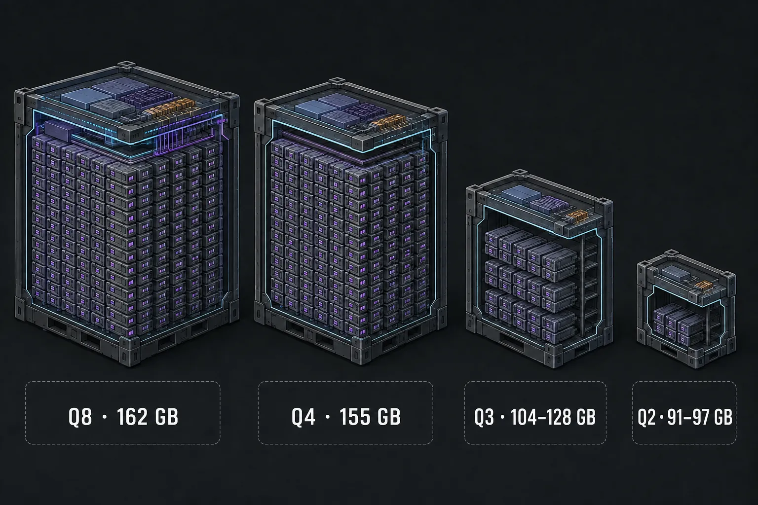
Four storage containers for Q8, Q4, Q3, and Q2 packages: the first two nearly identical in size because both keep the same four-bit expert mass; the smaller two visibly remove structure.

Against that baseline, DeepSeek-V4-Flash-0731’s listing looks broken:

Variant	Approximate size
UD-Q8_K_XL	162 GB
UD-Q4_K_XL	155 GB
Q3 variants (IQ3/Q3_K)	104–128 GB
IQ2/Q2 variants	91–97 GB
IQ1 variants	82–87 GB

Llama’s Q8 to Q4 step drops 32 GB, about 43% of the file. DeepSeek’s drops 7 GB, about 4%.

The intuition that fails is the one that assumes the starting point was high precision. Llama’s converter began with BF16 weights and genuinely had 16 bits to spend down. DeepSeek’s converter began with weights already at four bits, and a format-aware conversion doesn’t inflate native FP4 experts up to eight just because the package says “Q8” — it preserves the four-bit representation and spends the extra precision elsewhere. Nor can a Q4 conversion halve an expert population already sitting at roughly four bits.

So the gap between DeepSeek’s Q8 and Q4 lives almost entirely in the minority of the model: non-expert tensors, scales, metadata, runtime layout. The 304-billion-parameter bulk is the same four-bit experts in both files.

The sharpest way to hold these two side by side: both models ship mixed precision, but the causal direction is reversed. Llama’s mixture was layered on afterward by a quantizer author making judgment calls about which tensors to protect. DeepSeek’s was decided during training, and the weights were shaped around it. That difference is invisible in a filename and decisive for what you should expect.

How to think about each format

Official native mixed-precision checkpoint

About 167 GB, and the natural baseline whenever your runtime supports the required kernels. It gives you the intended reference quality, the precision layout the designers chose, native FP4 experts, block-scaled FP8 elsewhere, and higher precision on the operations that needed it.

Q8 or native-aware GGUF

About 162 GB. This exists for runtime compatibility; it cannot exceed the quality of the checkpoint it was made from. When the converter preserves the native FP4 expert structure and avoids pointless requantization, it stays very close to the source.

Unsloth describes its Q8 variant as lossless relative to the source. That’s the publisher’s characterization, not an independent benchmark across workloads.

Q4 or native-aware GGUF

About 155 GB, saving roughly 7 GB over Q8. The quality cost is probably small when the conversion mainly touches tensors that tolerate four bits well.

But look at what you’re trading. If your system already fits Q8, seven gigabytes is a rounding error against the uncertainty you take on about exactly which tensors got compressed and how.

Q3

Roughly 104–128 GB depending on the scheme. This is where the savings finally get real, and also where the converter starts requantizing tensors that were never designed for three-bit storage.

The first losses won’t show up in casual conversation. Look for them in code generation, agentic workflows, exact formatting, multilingual output, repository-scale retrieval, and long-context reasoning.

A Q3 model still sounds polished right up until you ask it for something exact.

Q2

Roughly 91–97 GB. At this level, real capability loss is a serious risk.

The model will likely keep its general fluency, broad factual associations, recognizable style, and plausible conversational manner, which is to say all the things that make a demo feel fine. Expect more failures in reasoning, retrieval, instruction adherence, and structured output. Without task-specific evaluation, don’t assume it matches the native checkpoint on anything that matters to you.

IQ1

Roughly 82–87 GB, and firmly experimental.

These preserve broad language behavior better than precise reasoning: the statistical structure behind fluent prose is forgiving, and exact symbolic operations are not. For architecture work, code generation, tool use, or agentic execution, where one wrong character can invalidate everything, that’s rarely the trade you want.

One honest caveat on all of the above: no rigorous, comprehensive public benchmark matrix evaluates every DeepSeek-V4-Flash-0731 quantization under identical settings. Quoting a figure like “Q3 loses 4.7% accuracy” would invent precision the evidence doesn’t support. The real loss depends on the implementation, the runtime, the workload, the prompt distribution, the context length, and the metric you score with.

Why one model’s Q4 can beat another model’s Q8

Bit count is a poor predictor across models. A four-bit model trained for four-bit execution can outperform a carelessly quantized eight-bit one, and here are the factors that decide it.

Was the precision native to training? A QAT-trained FP4 model spent its entire training run learning to work within four-bit constraints. A post-training INT8 model got rounded once, with no chance to adapt. The nominally smaller representation can be the more faithful one.

How large are the quantization groups? One scale for an entire tensor is crude: if that tensor holds both ordinary small values and a few enormous outliers, the single scale must stretch to cover the extremes, leaving almost no resolution for the values clustered near zero. Per-channel, per-128-value-group, or per-128×128-block scaling lets the representation follow local ranges closely. DeepSeek uses block scaling for its FP8 tensors.

How are outliers handled? Transformer tensors reliably contain a few unusually large values, and those few numbers can ruin the scale for the millions around them. Good quantizers keep outlier channels at higher precision, shrink the groups, choose clipping thresholds that minimize total error, or exclude certain tensors from aggressive compression entirely.

Which tensors were compressed? Not every component tolerates it equally. Large feed-forward expert matrices are comparatively safe. Router logits, attention query and key projections, normalization parameters, embeddings, output logits, and the KV cache are all riskier, and an average bit count tells you nothing about which of them got what treatment.

At what precision are results accumulated? This one is the most commonly overlooked. Four-bit inputs don’t mean four-bit arithmetic. A matrix multiplication sums thousands of products to produce each output value, and that running total is the accumulator. Good kernels multiply low-precision operands but accumulate into BF16 or FP32.

It’s the difference between rounding each item on a grocery receipt to the nearest dollar and rounding the running total to the nearest ten dollars after every single item. The first is a small error per item that largely averages out. The second compounds into nonsense. Keeping the accumulator wide preserves most of the answer even when the inputs are heavily compressed.

What “accuracy loss” should mean for your workload

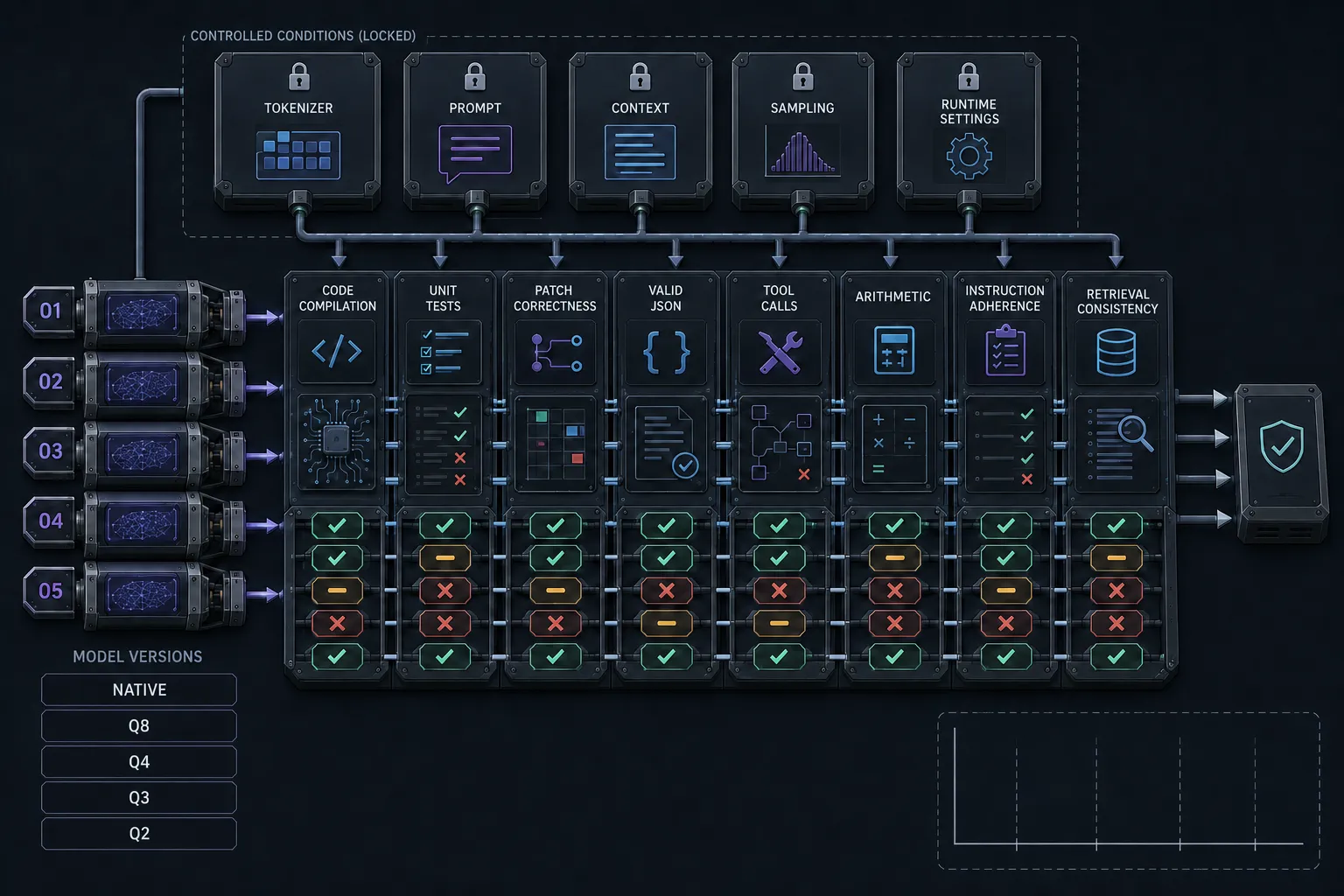
An evaluation workbench running five versions of one model through an identical locked pipeline of practical pass/fail stations — compilation, tests, JSON validity, tool calls, arithmetic, retrieval.

General benchmark averages are useful, but they don’t answer the question that decides a deployment:

Will this quantized model still do the work I need it to do?

Perplexity, a measure of how surprised the model is by text, is the standard quick check, and it’s close to useless here. It averages over ordinary tokens, which is exactly where quantization damage doesn’t show up. A model can hold its perplexity while its ability to close a JSON brace falls apart.

So skip the aggregate scores and measure outcomes on the work you actually run:

whether generated code compiles,
unit-test pass rates,
patch correctness,
exact JSON and tool-call validity,
instruction adherence,
repository-scale context retrieval,
recognition of subtle constraints,
arithmetic and symbolic correctness,
and consistency across repeated runs.

Then control the surroundings, because it’s easy to attribute a configuration difference to quantization. Hold constant the model revision, tokenizer, chat template, reasoning configuration, context length, prompt, sampling parameters, stop tokens, and runtime.

Run it twice. Start at temperature zero and score deterministic outcomes, then repeat with the sampling settings you’ll actually deploy. The two runs answer different questions, because quantization shifts the probabilities of close calls: a model that looks identical when you always take the top token can still behave less consistently once you’re sampling among near-ties.

For DeepSeek-V4-Flash-0731, a sensible ladder is:

Official native checkpoint
Q8 or native-preserving conversion
Q4 or native-preserving conversion
Best available Q3
Best available Q2

For a conventional model like Llama 3.3 70B the ladder is different, because the interesting rungs are elsewhere. Start at Q8_0, then walk down through Q6_K, Q5_K_M, and Q4_K_M, since that’s the stretch where the publisher stops saying “recommended” and your own tasks have to settle the question.

Push the same several hundred representative tasks through each, measure pass rates, and compute confidence intervals so you can tell a real regression from noise. Ten casual conversations will tell you almost nothing, for the reason established earlier: fluency is the last thing to go.

How to read a quantization label

For a conventional BF16 open-weight model, the kind Llama 3.3 70B represents, a reasonable broad expectation:

BF16 and FP16 — essentially reference quality
Well-implemented FP8 — often effectively reference quality
INT8 — usually a small degradation
Good weight-only INT4 — often highly usable, depending on workload
Three-bit — noticeably greater risk
Two-bit and below — substantial capability risk

Even there, the labels are approximations over a mixed interior. Q4_K_M stores closer to 4.8 bits per parameter than 4, and it protects the embedding and output layers on purpose. Someone made that call by hand after training.

DeepSeek-V4-Flash-0731 starts somewhere else entirely, and reading its labels with the conventional expectations produces exactly the wrong conclusions. Its reference checkpoint already combines FP4 routed experts, block-scaled FP8 through most of the remaining computation, dynamic activation quantization, and higher precision where it counts.

So: expanding those FP4 values into BF16 can’t reconstruct training weights that were never released. Q8 is a compatibility wrapper, not an upgrade. Q4 saves surprisingly little, because most of the model was already there. The degradation that actually matters begins further down, when a conversion pushes the non-expert tensors, the scaling metadata, or the KV cache toward three bits and below.

Which brings the whole thing back to the five questions the bit count can’t answer. What was quantized. How it was scaled. What stayed at higher precision. Whether the model was trained for the representation it ships in. And how it performs on the work you actually do.

Those are answerable. The config file, the model card, and the paper cover the first four, and a few hundred of your own tasks cover the fifth. It’s more effort than reading the number on the download, and it’s the only thing that tells you what you’re running.