Your Ten-Dimension Rubric Measures One Thing
- evals
- llm
- rubrics
- statistics
The comparison rubric in my evaluation harness scores ten named dimensions. Completeness, accuracy, understood intent, planning, execution, instruction fidelity, calibration, concision, depth, self-consistency. Ten axes, each with its own written definition, each judged separately, plotted as a radar chart with one polygon per model.
I built it that way for the obvious reason. A single score tells you a model is worse; ten scores are supposed to tell you how: this one rambles, that one skips constraints, the other is thorough but shallow. The whole appeal of a multi-axis rubric is that it turns a verdict into a diagnosis.
Here is the chart from a nine-model run.
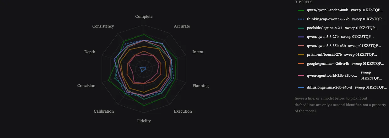
Nine polygons, nested like tree rings. Almost nothing crosses.
Across the nine models, the average correlation between any two of the ten dimensions is 0.973, and a single factor accounts for 97.6% of the variance in the whole ten-by-ten matrix. The chart has ten axes and roughly one axis worth of information on it.
By the end you should be able to answer:
- how to tell, from your own rubric scores, whether your axes are measuring different things,
- why the two axes most obviously in tension still correlate at 0.89,
- why instructing a judge to keep its criteria independent does not make them independent,
- what is actually left in a profile once you remove the part that is just “this model is better”,
- and how to plot a rubric so the shape means something.
The rule, up front: plot the residuals, not the scores. A radar chart of raw rubric scores is a picture of overall quality drawn ten times. Subtract each model’s own mean before you plot, and the small amount of genuine profile information becomes visible. The rest of this is why that is necessary and what it reveals.
Nested rings mean one variable
Look at the shape of the failure before the arithmetic, because the picture is unusually legible.
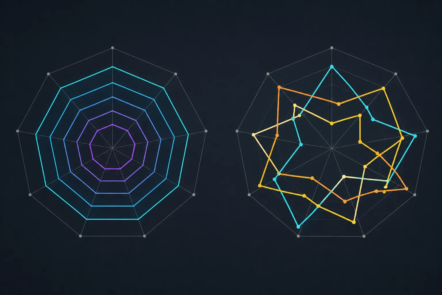
If ten axes measured ten different things, the polygons would cross. A model strong on concision and weak on depth would bulge on one side and pinch on the other; another model would do the reverse; their outlines would intersect. Crossings are what a profile looks like.
If ten axes measure one thing, the polygons nest. Every model’s outline sits wholly inside the next model up, because a single quantity, how good the judge thinks this model is, scales all ten radii together. Nesting is what a level looks like.
The chart above nests.
Here are the underlying numbers, sorted by overall score:
| Model | Compl. | Accur. | Intent | Plan. | Exec. | Fidel. | Calib. | Concis. | Depth | Consist. |
|---|---|---|---|---|---|---|---|---|---|---|
qwen3-coder-480b | 3.90 | 3.43 | 3.83 | 3.72 | 4.00 | 4.19 | 3.52 | 4.23 | 3.21 | 3.86 |
thinkingcap-qwen3.6-27b | 3.28 | 3.58 | 3.27 | 3.54 | 3.38 | 3.14 | 3.50 | 3.23 | 3.45 | 3.53 |
poolside/laguna-s-2.1 | 3.26 | 2.92 | 3.32 | 3.32 | 3.43 | 3.47 | 3.01 | 3.47 | 2.99 | 3.19 |
qwen/qwen3.6-27b | 3.26 | 3.55 | 3.29 | 3.11 | 3.18 | 3.01 | 3.28 | 2.88 | 3.57 | 3.25 |
qwen/qwen3.6-35b-a3b | 3.22 | 3.17 | 3.18 | 2.94 | 3.01 | 3.12 | 3.12 | 2.61 | 3.05 | 3.06 |
prism-ml/bonsai-27b | 2.54 | 2.83 | 2.57 | 2.68 | 2.56 | 2.67 | 2.74 | 2.51 | 2.78 | 2.72 |
google/gemma-4-26b-a4b | 2.02 | 1.88 | 2.02 | 2.01 | 1.77 | 1.69 | 2.02 | 2.02 | 1.94 | 1.87 |
agentworld-35b-a3b | 1.64 | 1.84 | 1.80 | 1.57 | 1.40 | 1.63 | 1.88 | 1.34 | 1.80 | 1.79 |
diffusiongemma-26b-a4b-it | 0.17 | 0.25 | 0.17 | 0.17 | 0.13 | 0.17 | 0.42 | 0.31 | 0.43 | 0.22 |
Read down any column. The order barely changes. Read across any row and the numbers cluster around that model’s overall level.
(These are not marks out of five. Like everything in this harness they are win rates in disguise. A 4.19 on an axis means “beats a typical rival about 84% of the time on that axis”. The nesting is not an artefact of the rescaling; it is present in the win rates themselves.)
The two axes that should have fought
There is a cheap way to dismiss all of this: good models are simply better at everything, so of course the axes correlate. Hold that thought, because it is a real objection and I will come back to it. First, test it where it is weakest.
Pick the two dimensions that are genuinely, structurally in tension. Concision rewards saying it in fewer words. Depth rewards going further into the material. You cannot maximise both without limit; past some point one is bought with the other. If any pair in this rubric should show a negative correlation, or at least no correlation, it is this one.
| Dimension pair | Correlation |
|---|---|
| concision ~ depth | 0.892 |
| accuracy ~ concision | 0.899 |
| instruction fidelity ~ depth | 0.925 |
| … | |
| accuracy ~ calibration | 0.995 |
| accuracy ~ depth | 0.997 |
| completeness ~ understood intent | 0.998 |
Concision and depth is the least correlated pair in the entire matrix, and it still sits at 0.892. Forty-three of the forty-five pairs exceed 0.9. Forty exceed 0.95.
The pair that should have been in opposition came out as the mildest agreement in the set. Whatever is driving these scores, it is not ten separate judgements about ten separate properties.
The rubric saw this coming and said so, in writing
The design already anticipated the problem, which is what makes this the most instructive part of the run. The rubric does not just list ten axes and ask for scores. It asks for eleven verdicts: the ten dimensions, plus a separate holistic overall. And it instructs the judge, in the prompt, that the overall verdict
is NOT a tally of the ten axes above and you must not compute it by counting wins. A response can lose most of the axes and still be the better answer — one broken constraint or one invented fact can outweigh ten small wins […] The ten and the overall are recorded separately on purpose, and where they disagree that disagreement is exactly what we want to see.
That is about as direct as an instruction gets. Do not collapse these. We are watching for the disagreement.
Across the nine models, the overall score correlates with the plain mean of the ten dimensions at r = 0.9954. Within individual prompts it averages 0.978.
The instruction did not survive contact with the forward pass.
To be fair to it, the effect is not literally zero. The overall verdict is not a pure copy of the dimension average: on eight of the twelve prompts, ranking the models by overall puts at least two of the nine in different positions than ranking them by the dimension mean. There is a little independent signal in there. There is just very little, and it is nowhere near the “a response can lose most of the axes and still be the better answer” behaviour the rubric was written to capture.
Eleven verdicts, one forward pass
The structural reason is visible in the plumbing. All eleven verdicts for a matchup come back from a single judge call on a single pair. One prompt goes out containing both answers and the full rubric; one reply comes back with eleven fields in it.
So these are not eleven measurements. They are one reading of one pair, partitioned eleven ways after the fact. Everything the model concluded in the first few hundred tokens of that reply, including which answer it liked, is in context for every field that follows. Asking the eleventh field to be independent of the first ten is asking a model to disregard its own visible reasoning.
The instruction is doing real work against a much stronger current.
Thorndike measured this in 1920
The phenomenon has a name and a hundred years of literature, and it did not start with language models.
In 1920 Edward Thorndike looked at ratings of aviation cadets by their commanding officers. The officers had rated each man on a set of supposedly independent traits: intelligence, physique, leadership, character. Thorndike found the correlations between trait pairs implausibly large and implausibly uniform, and of a second set of raters in the same paper he wrote that the correlations were “too high and too even”. A man rated well on one thing was rated well on all of them, with a regularity no genuine independence could produce. He concluded that the raters were not evaluating a compound of separate qualities at all; they had formed one global impression of each man and then spread it across the form. He called the error “the halo”, in scare quotes, as a term he was coining on the spot. The fixed phrase halo effect came later; what is in the 1920 paper is “a halo of general merit” spreading across every rating on the form.
An LLM judge handed a rubric is in the same position as those officers, with one difference that makes it worse: the officers at least filled in the form from memory over time, while the judge writes all eleven verdicts in one continuous generation with its own earlier words in front of it.
Recent work on LLM-judge rubric design names this directly. The Autorubric preprint lists “criterion conflation” as a failure mode, describing how judging multiple quality dimensions together causes the judgments to conflate distinct constructs, and its proposed remedy is to evaluate each criterion in a separate model call. That is a preprint rather than settled practice. It is also, independently, the same conclusion this run pushed me toward.
What is actually in the profile
Now the useful part. The general factor is not all there is. It is just so much larger that it hides everything else. Subtract each model’s own mean across the ten dimensions and the remainder is that model’s shape.
| Model | Compl. | Accur. | Intent | Plan. | Exec. | Fidel. | Calib. | Concis. | Depth | Consist. |
|---|---|---|---|---|---|---|---|---|---|---|
qwen3-coder-480b | +0.11 | −0.36 | +0.04 | −0.07 | +0.21 | +0.40 | −0.27 | +0.44 | −0.58 | +0.07 |
thinkingcap-qwen3.6-27b | −0.11 | +0.19 | −0.12 | +0.15 | −0.01 | −0.25 | +0.11 | −0.16 | +0.06 | +0.14 |
poolside/laguna-s-2.1 | +0.03 | −0.32 | +0.09 | +0.08 | +0.19 | +0.23 | −0.23 | +0.23 | −0.25 | −0.05 |
qwen/qwen3.6-27b | +0.03 | +0.31 | +0.05 | −0.13 | −0.06 | −0.23 | +0.05 | −0.36 | +0.33 | +0.01 |
qwen/qwen3.6-35b-a3b | +0.17 | +0.12 | +0.13 | −0.10 | −0.04 | +0.07 | +0.07 | −0.44 | +0.01 | +0.01 |
prism-ml/bonsai-27b | −0.12 | +0.17 | −0.09 | +0.02 | −0.10 | +0.01 | +0.07 | −0.15 | +0.12 | +0.06 |
google/gemma-4-26b-a4b | +0.10 | −0.05 | +0.09 | +0.09 | −0.15 | −0.24 | +0.10 | +0.09 | +0.02 | −0.06 |
agentworld-35b-a3b | −0.03 | +0.17 | +0.13 | −0.10 | −0.27 | −0.04 | +0.21 | −0.33 | +0.13 | +0.12 |
diffusiongemma-26b-a4b-it | −0.07 | +0.01 | −0.08 | −0.08 | −0.11 | −0.08 | +0.17 | +0.07 | +0.19 | −0.03 |
There is a real pattern here, and it is one you would never see on the raw chart.
qwen3-coder-480b is the terse one: +0.44 concision and +0.40 instruction fidelity against −0.58 depth and −0.36 accuracy. It hits the constraints and stops. qwen/qwen3.6-27b is close to its mirror image: −0.36 concision, +0.33 depth, +0.31 accuracy. It goes long and gets more right.
Those are genuinely different models to work with, and the difference is legible only after the level is removed. That is also the concision/depth tension the raw correlation could not find. It is there; it is just an order of magnitude smaller than the thing sitting on top of it.
How much smaller:
| Quantity | Spread |
|---|---|
| Raw dimension values across all models | 1.065 |
| The same values after subtracting each model’s own mean | 0.179 |
Six to one on the standard deviations, which is 97% against 3% once you square them into variances. Plot the raw values and almost everything you are looking at is the answer to “which model is better overall”, a question one number already answered and then drew ten times around a circle. That 97% is computed a different way from the 97.6% eigenvalue above, and the two agreeing is a decent sign neither is an artefact.
The objection I cannot rule out
Back to the cheap dismissal, because it deserves a straight answer.
A general factor is exactly what you would see if the judge cannot hold ten criteria apart. It is also exactly what you would see if model quality across this prompt set is genuinely close to one-dimensional — if the models that write more accurate answers really are the same models that plan better and follow instructions better, because all of those come from the same underlying capability.
This data cannot separate those two explanations. Doing so would need a design this study does not have: the same answers scored by independent judge calls per axis, or pairs constructed to be deliberately strong on one axis and weak on another, so you could check whether the rubric detects a difference you planted yourself.
I am not going to claim the halo explanation is proven. Both stories are live, and the honest position is that the rubric produced one number regardless of which is true.
What survives either way is the practical part. Whether the axes collapsed because of the judge or because model quality is genuinely correlated, a radar chart of raw scores is showing you a level and calling it a profile — and the fix is the same in both worlds.
What to do with your own rubric
Compute the correlation matrix before you trust the chart. It is one line of code over data you already have. If the mean off-diagonal correlation is above about 0.9, your axes are one axis and every conclusion you have drawn from the shape of that polygon is a conclusion about overall quality.
Centre each model before plotting. Subtract the model’s own mean across the axes and plot the residual. You lose the level, which you should report separately as the single number it always was, and you gain the shape, at a scale where it is visible.
Report the level and the profile as two claims. “This model is better” and “this model is terse relative to its own standard” are different findings with different evidence behind them. A single chart that fuses them will be read as the stronger of the two.
Do not expect a written instruction to enforce independence. Telling a judge that the overall verdict is not a tally is worth doing and it did measurably something here. It did not produce independence, and it will not, as long as eleven verdicts share one context window. If you need axes that do not contaminate each other, score them in separate calls and pay for it.
Test your rubric on planted contrasts. Construct a pair where one answer is deliberately terse and correct and the other is long and slightly wrong. If concision and depth do not separate on that pair, they will not separate on anything, and you have nine axes you can delete.
References
- Thorndike (1920), “A Constant Error in Psychological Ratings” — Journal of Applied Psychology 4(1):25–29; the aviation-cadet ratings, the “too high and too even” correlations, and Thorndike coining “the halo”
- Autorubric: Unifying Rubric-based LLM Evaluation — preprint; “criterion conflation” as a named failure mode of single-call multi-criterion judging, and per-criterion decomposition as the proposed remedy
The rubric text, the scores, and the judge plumbing quoted here come from a private evaluation harness on my own machine and are not linkable. The correlation matrix, the first-eigenvalue share, and the residual table are computed directly from that run’s stored record.